Using Environments

The goal of Ecole is to provide Markov decision process abstractions of common sequential decision making tasks that appear when solving combinatorial optimization problems using a solver. These control tasks are represented by stateful classes called environments.

In this formulation, each solving of an instance is an episode. The environment class must first be instantiated, and then a specific instance must be loaded by a call to reset(), which will bring the process to its initial state. Afterwards, successive calls to step() will take an action from the user and transition to the next state. Finally, when the episode is finished, that is when the instance has been fully solved, a new solving episode can be started with another call to reset().

For instance, using the Branching environment for branch-and-bound variable selection, solving a specific instance once by always selecting the first fractional variable would look as follows.

import ecole

env = ecole.environment.Branching()
env.seed(42)

for _ in range(10):
    observation, action_set, reward_offset, done, info = env.reset("path/to/instance")
    while not done:
        observation, action_set, reward, done, info = env.step(action_set[0])

Let us analyze this example in more detail.

General structure

The example is driven by two loops. The inner while loop, the so-called control loop, transitions from an initial state until a terminal state is reached, which is signaled with the boolean flag done == True. In Ecole, the termination of the environment coincides with the termination of the underlying combinatorial optimization algorithm. A full execution of this loop is known as an episode. The control loop matches a Markov decision process formulation, as used in control theory, dynamic programming and reinforcement learning.

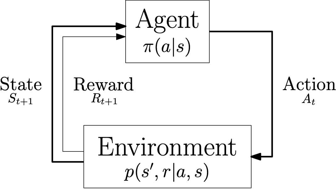
The control loop of a Markov decision process.

Note

More exactly, the control loop in Ecole is that of a partially-observable Markov decision process (PO-MDP), since only a subset of the MDP state is extracted from the environment in the form of an observation. We omit this detail here for simplicity.

The outer for loop in the example simply repeats the control loop several times, and is in charge of generating the initial state of each episode. In order to obtain a sufficient statistical signal for learning the control policy, numerous episodes are usually required for learning. Also, although not showcased here, there is usually little practical interest in using the same combinatorial problem instance for generating each episode. Indeed, it is usually desirable to learn policies that will generalize to new, unseen instances, which is very unlikely if the learning policy is tailored to solve a single specific instance. Ideally, one would like to sample training episodes from a family of similar instances, in order to solve new, similar instances in the future. For more details, see the Ecole theortical model in the discussion.

Environment parameters

Each environment can be given a set of parameters at construction, in order to further customize the task being solved. For instance, the Branching environment takes a pseudo_candidates boolean parameter, to decide whether branching candidates should include all non fixed integral variables, or only the fractional ones. Environments can be instantiated with no constructor arguments, as in the previous example, in which case a set of default parameters will be used.

Every environment can optionally take a dictionary of SCIP parameters that will be used to initialize the solver at every episode. For instance, to customize the clique inequalities generated, one could set:

env = ecole.environment.Branching(
    scip_params={"separating/clique/freq": 0.5, "separating/clique/maxsepacuts": 5}
)

Warning

Depending on the nature of the environment, some user-given parameters can be overriden or ignored (e.g., branching parameters in the Branching environment). It is the responsibility of the user to understand the environment they are using.

Note

For out-out-the-box strategies on presolving, heuristics, and cutting planes, consider using the dedicated SCIP methods (SCIPsetHeuristics etc.).

Observation functions and reward functions are more advanced environment parameters, which we will discuss later on.

Resetting environments

Each episode in the inner while starts with a call to reset() in order to bring the environment into a new initial state. The method is parameterized with a problem instance: the combinatorial optimization problem that will be loaded and solved by the SCIP solver during the episode. In the most simple case this is the path to a problem file. For problems instances that are generated programatically (for instance using PyScipOpt or using instance generators) a ecole.scip.Model is also accepted.

• The observation consists of information about the state of the solver that should be used to select the next action to perform (for example, using a machine learning algorithm.) Note that this entry is always None when the state is terminal (that is, when the done flag described below is True.)

• The action_set, when not None, describes the set of candidate actions which are valid for the next transition. This is necessary for environments where the action set varies from state to state. For instance, in the Branching environment the set of candidate variables for branching depends on the value of the current LP solution, which changes at every iteration of the algorithm.

• The reward_offset is an offset to the reward function that accounts for any computation happening in reset() when generating the initial state. For example, if clock time is selected as a reward function in a Branching environment, this would account for time spent in the preprocessing phase before any branching is performed. This offset is thus important for benchmarking, but has no effect on the control problem, and can be ignored when training a machine learning agent.

• The boolean flag done indicates whether the initial state is also a terminal state. This can happen in some environments, such as Branching, where the problem instance could be solved though presolving only (never actually getting to branching).

See the reference section for the exact documentation of reset().

Transitioning

The inner while loop transitions the environment from one state to the next by giving an action to step(). The nature of observation, action_set, and done is the same as in the previous section Resetting environments. The reward and info variables provide additional information about the current transition.

See the reference section for the exact documentation of step().

Seeding environments

Environments can be seeded by using the seed() method. The seed is used by the environment (and in particular the solver) for all the subsequent episode trajectories. The solver is given a new seed at the beginning of every new trajectory (call to reset()), in a way that preserves determinism, without re-using the same seed repeatedly.

See the reference section for the exact documentation of seed().